Method of Computing Link Relative Ratio and Year-on-year Comparison in R Language

Cross-row and –group computation often involves computing link relative ratio and year-on-year comparison. Link relative ratio refers to comparison between the current data and data of the previous period. Generally, it takes month as the time interval. For example, compare the sales amount of April with that of March, and the growth rate we get is the link relative ratio of April. Hour, day, week and quarter can also be used as the time interval. Year-on-year comparison is the comparison between the current data and data of the corresponding period of the previous year. For example, compare the sales amount of April 2014 with that of April 2013 and compute the growth rate which is April's year-on-year comparison. Data of multiple periods are usually compared to find the variation trend in practical business.

Now let's look at the method of computing link relative ratio and year-on-year comparison in R language through an example.

Case description:

Compute the link relative ratio and year-on-year comparison of each month's sales amount during a specified period of time. The data come from orders table sales, in which column Amount contains order amount and column OrderDate contains order dates. Some of the data are as follows:

Code:
sales<-read.table("E:\\ salesGroup.txt",sep="\t", header=TRUE)
filtered<-subset(sales,as.POSIXlt(OrderDate)>=as.POSIXlt('2011-01-01 00:00:00') &as.POSIXlt(OrderDate)<=as.POSIXlt('2014-08-29 00:00:00'))
filtered$y<-format(as.POSIXlt(filtered$OrderDate),'%Y')
filtered$m<-format(as.POSIXlt(filtered$OrderDate),'%m')
agged<-aggregate(filtered$Amount, filtered[,c("m","y")],sum)
agged$lrr<- c(0, (agged$x[-1]-agged$x[-length(agged$x)])/agged$x[-length(agged$x)])
result<-agged[order(agged$m),]
result$yoy<-NA
for(i in 1:nrow(result)){
if(i>1 && result[i,]$m==result[i-1,]$m){
result[i,]$yoy<-(result[i,]$x-result[i-1,]$x)/result[i-1,]$x
}
}
Code interpretation:
1. The first four lines of code are easy to understand. read.table is used to read data from the table and subset to filter data, and two format functions are used to generate year and month respectively. Note that the beginning and ending time should be output dynamically from the console using scan function; here they are simplified as fixed constants.

After computing, some of the values of database frame filtered are:

2. agged<-aggregate(filtered$Amount, filtered[,c("m","y")],sum), this line of code summates the order amount of each month of each year. Note that in the code, the month must be written before the year though data are grouped by the year and the month according to business logic. Otherwise R language will perform grouping first by the month, then by the year, which will get result inconsistent with business logic and make data viewing inconvenient.

After computing, some of the values of data frame agged are:

3. agged$lrr<- c(0, (agged$x[-1]-agged$x[-length(agged$x)])/agged$x[-length(agged$x)])，this line of code computes link relative ratio. The result will be stored in the new column Irr. Business logic is (order amount of the current month – order amount of the previous month)\order amount of the previous month.

Note: [-N] in the code represents that the Nth row of data is removed. So agged$x[-1]means the first row of data is removed and agged$x[-length(agged$x)]means the last row of data is removed. By performing certain operation between the two, link relative ratio can be obtained indirectly. But the result won’t include the link relative ratio of the first month (i.e. January 2011), so a zero should be added to the code. We can see that the code logic and the business logic share some similarities but are quite different. The code is difficult to understand.

At this point, some of the values of data frame aggedare:

4. result<-agged[order(agged$m),], this line of code sorts data by the month and the year. Since the data of the year are ordered, we just need to perform sorting by the month. result$yoy<-NA initializes a new column which will be used to store the year-on-year comparison of sales amount.

Now the value of result is:

5. The loop judgment in the last four lines of code is to compute the year-on-year comparison. Business logic: (order amount of the current month – order amount of the previous month)\order amount of the previous month. Code logic: from the second line, if the month in the current line is the same as that in the previous line, the code will compute year-on-year comparison. Detailed code is result[i,]$yoy<-(result[i,]$x-result[i-1,]$x)/result[i-1,]$x. We can see that the code written in this way is easy to understand and its logic is quite similar to the business logic.

The only weakness of this piece of code is that it cannot use the loop function of R language, which makes it a little lengthy. But compared with the difficult operation of link relative ratio, maybe a longer but simple code is better.

The final results are as follows:

Summary:R language can compute link relative ratio and year-on-year comparison, but the operation of link relative ratio is difficult to understand and the code of year-on-year comparison is a little lengthy. The codes of both operations are not easy to learn.

The third-party solution

Python, esProc and Perl, all of which can perform structured data computation, can be used to handle this case. In the following, we'll briefly introduce esProc and Python's solutions.

esProc

esProc is good at expressing business logic freely with agile syntax. Its code is concise and easy, as shown below:

In the above code, groups function is used to group and summarize data by the year and the month. The derive functions in A4 and A6 generate link relative ratio and year-on-year comparison respectively.

As can be seen from the code, esProc also uses[-N]. Different from [-N] in R language, it doesn't represent removing the Nth row; it represents the Nth row counted from the current line. For example, [-1] is the previous line. In this way, the operation of link relative ratio can be simply expressed as (x-x[-1])/x[-1].But R language hasn't expressions for relative positions, which makes its code difficult to understand.

In the year-on-year comparison operation, esProc uses judgment function if in loop function, making it avoid the lengthy loop statement and its code simpler. While R language only has the judgment statement but hasn't the judgment function. This is the reason why its code is lengthy.

Finally, these are the computed results:

Python（Pandas）
Pandas is Python's third-party package. Its basic data type is created by imitating R’s dataframe but gets improved greatly. At present, its latest version is 0.14. Its code for handling this case is as follows:

sales = pandas.read_csv('E:\\salesGroup.txt',sep='\t')
sales['OrderDate']=pandas.to_datetime(sales.OrderDate,format='%Y-%m-%d %H:%M:%S')
filtered=sales[(sales.OrderDate>='2011-01-01 00:00:00') & (sales.OrderDate<='2014-08-29 00:00:00')]
filtered['y']=filtered.OrderDate.apply(lambda x: x.year)
filtered['m']=filtered.OrderDate.apply(lambda x: x.month)
grouped=filtered.groupby(['y','m'],as_index=False)
agged=grouped.agg({'Amount':[sum]})
agged['lrr']=agged['Amount'].pct_change()
result=agged.sort_index(by=['m','y'])
result.reset_index(drop=True,inplace=True)
result['yoy']=result.apply(lambda _:numpy.nan, axis=1)
for row_index, row in result.iterrows():
if(row_index>0 and result.ix[row_index,'m']==result.ix[row_index-1,'m']):
result.ix[row_index,'yoy']=(result.ix[row_index,'Amount']-result.ix[row_index-1,'Amount'])/result.ix[row_index-1,'Amount']

In the code, pct_change() function is used to directly compute the link relative ratio, which is more convenient than the method used by R language and esProc. But this kind of function is not universal and can only deal with isolated cases. When it is required to compute link relative ratio or year-on-year comparison, Pandas can only complete the task by combining div function and shift function, which makes its code more difficult to understand than R’s.

In computing year-on-year comparison, Pandas' code is as lengthy as R’s. This is because Pandas also cannot use if function in loop function. I’m afraid cooperation of apply function and lambda syntax is needed if we want to write simpler code.

Finally, let's look at the computed results:

Please pay attention to the following easy-to-get-wrong details:

1. The code must be sort_index(by=['m','y'])when we perform sorting by the month and the year. The simple form sort(m), which used in R language and esProc, is not allowed.

2. Pandas has the assignment syntax as result.loc[row_index,‘yoy’]=value. But when assigning value to a certain element in data frame, we should write the code as result.ix[row_index,'yoy']=value.

3.  When iterrows() is used to perform loop, its loop number row_index is index instead of row number. To make the row number conform to the index, reset_index() should be used to reset the indexes.

Comparison of Loop Function in esProc and R Language

Loop function can traverse every member of an array or a set, express complicated loop statements with simple functions, as well as reduce the amount of code and increase readability. Both esProc and R language support the loop function. The following will compare their similarities and differences in usage.

1.  Generating data

Generate odd numbers between 1 and 10.

esProc:

         x=to(1,10).step(2)            

In the code, to(1,10)generates consecutive integers from 1 to 10, step function gets members inconsecutively according to the computed result of last step and the final result is [1,3,4,5,7,9]. This type of data in esProc is called a sequence.

The code has a simpler version: x=10.step(2).

R language:

         x<-seq(from=1,to=10,by=2)    

This piece of code gets integers directly and inconsecutively from 1 to 10. Computed result is c(1,3,4,5,9). This type of data in R language is called vector.

A simpler version of this piece of code isx<-seq(1,10,2).

Comparison:

1.   Both can solve the problem in this example. esProc needs two steps to solve it, indicating theoretically a poor performance. While R language can resolve it with only one step, displaying a better performance.

2.   The method for esProc to develop code is getting members from a set according to the sequence number. It is a common method. For example, there is a string sequence A1=["a", "bc", "def"……],now get strings in the positions of odd numbers. Here it’s no need to change the type of code writing, the code isx=A1.step(2).
R language generates data directly, thus it has a better performance. It can write common expressions, too. For example, get strings in the positions of odd numbers from the string vector quantity A1=c("a", "bc", "def"……), the expression in R language can bex=A1[seq(1,length(A1),2)].

3. esProc loop function has characteristics that R language hasn't, that is, built-in loop variables and operators. "~" represents the loop variable, "#" represents the loop count, "[]" represents relative position and “{}” represents relative interval. By using these variables and operators, esProc can produce common concise expressions. For example, seek square of each member of the set A2=[2,3,4,5,6]:

         A2.(~*~)                              /Result is[4,9,16,25,36], which can also be written as A2**A2. But the latter lacks a sense of immediacy and commonality.R language can only use A2*A2 to express the result.

         Get the first three members:

         A2.select(#<=3)                 / Result is [2,3,4]

         Get each member’s previous member and create a new set:

         A2.(~[-1])                             / Result is [null,2,3,4,5]

         Growth rate:

         A2.((~ - ~[-1])/ ~[-1])         /Result is [null,0.5,0.33333333333,0.25,0.2]

         Moving average:

         A2.(~{-1,1}.avg())               /Result is [2.5, 3.0, 4.0, 5.0, 5.5]

Summary:In this example, that R language can directly generate data and produce common expressions shows that it is more flexible and takes less memory space than esProc.

2.  Filtering records

Computational objects of a loop function can be an array or a set whose members are single value, or two-dimensional structured data objects whose members are records. In fact, loop function is mainly used in processing the latter. For example, select orders of 2010 whose amount is greater than 2,000 from sales, the order records.
Note: sales originates from a text file, some of its data are as follows: 

esProc:

sales.select(ORDERDATE>=date("2010-01-01") && AMOUNT>2000)

Some of the results are:

R language:

sales[as.POSIXlt(sales$ORDERDATE)>=as.POSIXlt("2010-01-01") &sales$AMOUNT>2000,]

Some of the results are:

Comparison:

1.Both esProc and R language can realize this function. Their difference lies that esProc uses select loop function while R language directly uses index. But there isn’t an essential distinction between them. In addition, R language can further simplify the expression by using attach function:

sales[as.POSIXlt(ORDERDATE)>=as.POSIXlt("2010-01-01") & AMOUNT>2000,]

Thus, there are more similarities between them.    

     

2.  Except query, loop function can be used to seek sequence number, sort, rank, seek Top N, group and summarize, etc. For example, seek sequence numbers of records.

         sales.pselect@a(ORDERDATE>=date("2010-01-01") && AMOUNT>2000)   /esProc

         which(as.POSIXlt(sales$ORDERDATE)>=as.POSIXlt("2010-01-01") &sales$AMOUNT>2000) #R language

For example, sort records by SELLERID in ascending order and by AMOUNT in descending order.

         sales.sort(SELLERID,AMOUNT:-1)                              /esProc

         sales[order(sales$SELLERID,-sales$AMOUNT),]    /R language

For example, seek the top three records by AMOUNT.

         sales.top(-AMOUNT;3)                                                   /esProc

         head(sales[order(-sales$AMOUNT),],n=3)               /R language

3.  Sometimes, R language computes with index, like filtering; sometimes it computes with functions, like seeking sequence numbers of records; sometimes it programs in the form of “data set + function + data set”, like sorting; and other times it works in the way of “function + data set + function”, like seeking TopN. Its programming method seems flexible but is liable to greatly confuse programmers. By comparison, esPoc always adopts object-style method “data set + function + function …”in access. The method has a simple and uniform structure and is easy for programmers to grasp.

Here is an example of performing continuous computations. Filter records and seek Top N. esProc will compute like this:

sales.select(ORDERDATE>=date("2010-01-01") && AMOUNT>2000).top(AMOUNT;3)

And R language will compute in this way:

         Mid<-sales[as.POSIXlt(sales$ORDERDATE)>=as.POSIXlt("2010-01-01") &sales$AMOUNT>2000,]

         head(Mid [order(Mid$AMOUNT),],n=3)

As you can see, esProc is better at programming multi-step continuous computations.

Summary:In this example, esPoc gains the upper hand in ensuring syntax consistency and performing continuous computations, and is more beginner-friendly.

3.  Grouping and summarizing

The loop function is often employed in grouping and summarizing records. For example, group by CLIENT and SELLERID, and then sum up AMOUNT and seek the maximum value.

esProc:

         sales.groups(CLIENT,SELLERID;sum(AMOUNT),max(AMOUNT))

Some of the results are as follows:

R language:

         result1<-aggregate(sales[,4],sales[c(3,2)],sum) 

         result2<-aggregate(sales[,4],sales[c(3,2)],max)

         result<-cbind(result1,result2[,3])

Some of the results are as follows:

Comparison:

1. In this case, more than one summarizing method is required. esProc can complete the task in one step. R language has to go through two steps to sum up and seek the maximum value, and finally, combine the results with cbind, because its built-in library function cannot directly use multiple summarizing methods simultaneously. Besides, R language will have more memory usage in completing the task.

2.  Another thing is the illogical design in R language. For sales[c(3,2)], the group order in the code is that SELLERID is ahead of CLIENT, but in business, the order is completely opposite. In the result, the order changes again and becomes the same as that in the code. In a word, there is not a unified standard for business logic, the code and the computed result.

Summary:In this example, esProc has the advantages of high efficiency, small memory usage and having a unified standard.

4. Seeking quadratic sum

Use a loop function to seek quadratic sum of the set v=[2,3,4,5].

Please note that both esProc and R language have functions to seek quadratic sum, but a loop function will be used here to perform this task.

esProc:

v.loops(~~+~*~;0)

R language:

Reduce(function(x,y) x+y*y, c(0,v))

Comparison:

1. Both esProc and R language can realize this function easily.

2.   The use of loops function by esProc means that it sets zero as the initial value, computes every member of v in order and returns the final result. In the code, "~" represents member being computed and "~~" represents computed result of last step. For example, the arithmetic in the first step is 0+2*2 and that in the second step is4+3*3, and so forth.The final result is 54.

The use of reduce function by R language means that it computes members of [0,2,3,4,5] in order, and puts the computed result of the current step into the next one to go on with the computation. As esProc, the arithmetic in the first step is 0+2*2 and that in the second step is 4+3*3, and so forth.

3. R language employs lambda expression to perform the operation. This is one of the programming methods of anonymous functions, and can be directly executed without specifying the function name. In this example, function(x,y),the specification, defines two parameters; x+y*y, the body, is responsible for performing the operation; c(0,v) combines 0 and v into[0,2,3,4,5] in which every member will take part in the operation in order. Because it can input a complete function, this programming method becomes quite flexible and is able to perform operations containing complicated functions.

The esProc programming method can be regarded as an implicit lambda expression, which is essentially the same as the explicit expression in R language. But it has a bare expression without function name, specification and variables and its structure is simpler. In this example, “~” represents the built-in loop variable unnecessary to be defined; ~~+~*~is the expression responsible for performing the operation; v is a fixed parameter in which every member will take part in the operation in order. Being unable to input a function, it is not as good as R language theoretically in flexibility and ability of expression.

4. Despite being not flexible enough in theory, esProc programming method boasts convenient built-in variables and operators, like ~, ~~, #, [], {}, etc., and gets a more powerful expression in practical use. For example, esProc uses“~~” to directly represent the computed result of last step, while R language needs reduce function and extra variables to do this. esProc can use “#” to directly represent the current loop number while R language is difficult to do this. Also, esProc can use “[]”to represent relative position. For example, ~[1]is used to represent the value of next member and Close[-1]is used to represent value of the field Close in the last record.

In addition, esProc can use“{}”to represent relative interval. For example, {-1,1}represents the three members between the previous and next member. Therefore,the common expression v.(~{-1,1}.avg())can be used to compute moving average, while R language needs specific functions to do this. For example,there is even no such a function for “seeking average” in the expression filter(v/3, rep(1, 3),sides = 1), which is difficult to understand for beginners.

Summary:In this case, the lambda expression in R language is more powerful in theory but is a little difficult to understand. By comparison, esProc programming method is easier to understand.

5. Inter-rows and –groups operation

Here is a table stock containing daily trade data of multiple stocks. Please compute daily growth rate of closing price of each stock.

Some of the original data are as follows:

esProc:

         A10=stock.group(Code)

         A11=A10.(~.sort(Date))

         A12=A11.(~.derive((Close-Close[-1]):INC))

R language:

A10<-split(stock, stock $Code)

for(I in 1:length(A10){

         A10[[i]][order(as.numeric(A10[[i]]$Date)),] #sort by Date in each group

         A10[[i]]$INC<-with(A10[[i]], Close-c(0,Close[- length (Close)])) #add a column, increased price

}

Comparison:

1.  Both esProc and R language can achieve the task. esProc only uses loop function in computing, achieving high performance and concise code. R language requires writing code manually by using for statement, which brings poor performance and readability.

2.   To complete the task, two layers of loop are required: loop each stock, and then loop each record of the stocks. Except being good at expressing the innermost loop, loop function of R language (including lambda syntax) hasn't built-in loop variables and is hard to express multi-layer loops. Even if it manages to work out the code, the code is unintelligible.

Loop function of esProc can not only use “~” to represent the loop variable, but also be used in nested loop, therefore, it is expert at expressing multi-layer loops. For example, A10.(~.sort(Date))in the code is in fact the abbreviation of A10.(~.sort(~.Date)).The first “~” represents the current stock, and the second “~” represents the current record of this stock.

3.   As a typical ordered operation, it is required that the closing price of last day be subtracted from the current price. With the useful built-in variables and operators, such as #,[] and {}, esProc is easy to express this type of ordered operation. For example, Close-Close[-1]can represent the increasing amount. R language can also perform the ordered operation, but its syntax is much too complicated due to the lack of facilities like loop number, relative position, relative interval and so on. For example, the expression of increasing amount is Close-c(0,Close[- length (Close)]).

It is hard enough for loop function in R language to perform the relative simple ordered operation in this example, let alone the more complicated operations. In those cases, multi-layer for loop is usually needed. For example, find out how many days the stock has been rising:

A10<-split(stock, stock $Code)

for(I in 1:length(A10){

         A10[[i]][order(as.numeric(A10[[i]]$Date)),] #sort by Date in each group

         A10[[i]]$INC<-with(A10[[i]], Close-c(0,Close[- length (Close)])) #add a column, increased price

         if(nrow(A10[[i]])>0){  #add a column, continuous increased days

                   A10 [[i]]$CID[[1]]<-1

         for(j in 2:nrow(A3[[i]])){

         if(A10 [[i]]$INC[[j]]>0 ){

                 A10 [[i]]$CID[[j]]<-A10 [[i]]$CID[[j-1]]+1

         }else{

                 A10 [[i]]$CID[[j]]<-0

               }

             }   

           }

}

The code in esProc is still concise and easy to understand:

         A10=stock.group(Code)

         A11=A10.(~.sort(Date))

A12=A11.(~.derive((Close-Close[-1]):INC), if(INC>0,CID=CID[-1]+1, 0):CID))

Summary:In performing multi-layer loops or inter-rows and -groups operations, esProc loop function has higher computational performance and more concise code.

Comparison Between esProc’s Sequence Table Object and R’s Data Frame part(II)

Advanced features

Example 5: modifying the association. A1, A2 are two-dimensional structured data object with the same field ID. We now need to add the bonus field values of A2 to the salary field values ​​in A1 according to ID.

         Sequence table:

         A1=db.query("select id,name,salary from salary order by id")

         A2=db.query("select id,bonus from bonus order by id")

A1.modify(1:A2,salary+bonus:salary)              

         Data frame has no functions to modify the association. We need to do manual coding for this, which is omitted here.

Example 6: merging associations. A1, A2, A3 are two-dimensional structured data objects with the same field sequence number. Please associate them with left join. As the data is sorted by sequence number, please leverage merging methods to improve the speed for association.

Sequence Table：join@m1(A1:salary,id;     A2:bonus,id;   A3,attendance,id)

Data frame supports association of two tables, such as:     merge(A1,A2,by.x="id",by.y="id",all=TRUE).

In this case three tables are associated, which can be achieved indirectly through two two-table associations.

n addition, the data frame does not support merging of association, and therefore no speed improvement is possible. In other words, data frame cannot use ordered sequence data to improve performance, not only with association, but also with other operations.

Example 7: Record lookup. Four scenarios: retrieving records with the Amount greater than 1000; retrieving the sequence number or records with the Amount greater than 1000;return records with primary key value of “v”, return the sequence number for records with primary key value of “v”.

         Sequence table:

    =data.select(Amount>1000)  

    = data.pselect(Amount>1000)        

    = data.find(v)           

    = data.pfind(v)         

         Data frame：only the first two scenarios can be achieved, which is done with following code:

    newdata<- data [data $ Amount>1000,]        

which(data $ Amount >1000) 

Data frame hasn't the concept of major key, so we need to do manual coding for other 2 scenarios as indirect methods, or employ a third party package (i.e. data.table). The codes are omitted here.

Example 8: Group sum. The data is grouped by Client and SellerId. Then the other two fields are aggregated: do a sum for Amount field, and do a count for OrderID field.

Sequence table：

         =data.groups(Client,SellerId;sum(Amount),count(OrderID))

Data frame：only support single field aggregation, such as the sum of Amount. As following：

         result<aggregate(data[,4],data[c(2,3)],sum)

To do aggregation of two fields at the same time with data frame, we can only use two separate aggregate statements and then merge the results. Codes are omitted here.

Example 9: Reuse grouping. Group data by Client. Complete multiple subsequent computations on group result. Including: aggregation by amount, and count after grouping by SellerId.

Sequence table:

         A2=data.group(Client)

         =A2.(~.sum(Amount))

         =A2.(~.groups(SellerId;count(OrderID)))

Data frame does not support reuse of grouping directly. Grouping and aggregation usually need to be done in one step. This means we need to do two identical grouping operations to accomplish the same purpose. As following:

         result<-aggregate(data[,2],sum)

         result<-aggregate(data[,2],data[,3],count)

If we want to reuse grouping, we must use split function and loop to achieve this. The code is both lengthy and with low performance.

Summary:Sequence tables and data frame are quite different in terms of advanced features. This is mainly demonstrated in the following five ways:

1.       Richness of features. Sequence table has rich functions, and is very convenient to do structured data computation. Data frame originates from matrix, with less support for structured data and lack of many features. Use of the third party packages can in some degree supplement the functions data frame lacks, but these packages are no match for R’s primitive library function in muturity and stability.

2.       Difficulty in syntax. The function names of sequence table are more intuitive.For example, select means to find; pselect is to find the location (position). With data frame the syntax is relatively obscure. For example, “find by field” is data [data $ Amount> 1000,], and retrieve value by field is data[,"Amount"]. These two are confusing and difficult for the programmer to understand. One must have some knowledge on vector to grasp it.

3.       Memory consumption. Basically sequence table function only returns a reference, with very little memory occupation. Data frame must copied record from the original object. If we need to do multiple search, association and grouping operations on large amounts of data, data frame’s memory consumption will be very large. It will impact the whole system.

4.       Code workload and code performance. The functions supported by data frame are not rich enough. We need to do hand-coding to achieve this indirectly. This means more workload. The R interpreter is known to be very slow. With hand-coding the performance is much lower than library functions.

5.       Library function performance. Sequence table has many functions to improve computing performance, such as merging association, grouping functions, binary search, hash lookup. Although data frame supports association, aggregation and search, it’s hard to improve the performance.

Actual case

In this part we use a real case for comprehensive comparison o fdata frame and sequence table.
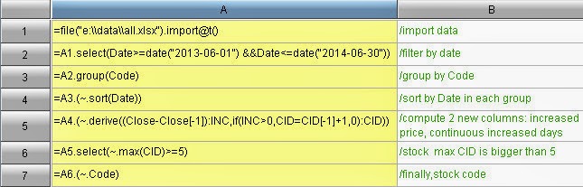
Computation target: according to daily transactions, selecting stocks from blue-chip stocks whose prices rises in 5 days in a row.
Ideas: Importing data; filtering out previous month's data; grouped them according to the ticker; sort the data by dates; compute the growth amount for closing price over previous day; compute the number of days for continuous positive growth; filtering out the stocks which rise in 5 or more days in a row.

Sequence Table:

Data frame:

Comparison：

1.       Data frame function is not rich enough, and is lack of professionalism. We need to use nested loops to meet the requirement in this case. It’s of low computational efficiency. Sequence table has rich and diverse functions. Without the use of loop statement we can achieve the same purpose. The code is shorter and simpler, and the performance is higher.

2.       When programming for data frame, the code is obscure and hard to write. With sequence table, the code is clear and easy to understand. The cost of learning is lower.

3.       When large amount of data is involved in this scenario, the memory consumption will be huge. Sequence table is computation by reference, which consumes less memory. Data frame is computation by value pass. The memory consumption is several times more than sequence table. It easy to result into memory overflow in this scenario.

4.       To import Excel data into data frame, R requires third-party software packages. However they seem to have difficulty working together. Data import needs ten minutes to complete. With sequence table this only needs tens of seconds.

Test Performance

Test 1: Generating 10 million records in memory, each consists of three fields. All values ​​are random numbers. Records are filtered, and each field is summed.

Sequence table:

Data frame：

Comparison: sequence table needs 50.534 seconds, while data frame needs 91.999 seconds. The gap is obvious.

Test 2: Retrieving 1.2G txt file. Do filtering and sum on two fields

Sequence Table

Data frame

Comparison: sequence table takes 87.122 seconds, while data frame takes 1.1347 hours. The performance difference is tens of times. The reason for this is mainly due to the extremely low speed for file reading.

From the above comparison, we can see that sequence table are better than data frame in terms of rich features, easy syntax, memory consumption, development effort, library function performance and coding performance, etc.. Of course, data frame is not the full strength of R language. R has a powerful vector matrix and the associated mass functions, which make it more professional than esProc in scientific and engineering computation. 

Comparison Between esProc’s Sequence Table Object and R’s Data Frame part(I)

Both esProc and R language are typical data processing and analysis languages with two-dimensional structured data objects. They are all good at multi-step complex computations. However their two-dimensional structured data objects are quite different from each other in the underlying mechanism. As a result, esProc is better at computation with structured data, and especially suitable for developers to do business computing. R is better at matrix computation and more suitable for scientists to do scientific or engineering computation.

esProc's two-dimensional structured data type is sequence table object (TSeq). Sequence table is based on records, with multiple records forming a row-styled two-dimensional table. In combination with the column name, this two-dimensional table can form a complete data structure. R language is based on vector, with multiple vectors forming a column-styled two-dimensional table. In combination with the column name, the two-dimensional table can form a complete data structure.

These underlying mechanisms affect actual user experience. In the following part we will compare the difference in practical use between sequence table object and data frame, in terms of basic functions, advanced features, actual use cases and test results.

Note: Primitive functions of development language are to be used in the following comparisons, the third party extension packages won’t be involved.

Basic functions

Example 1:retrieve two-dimensional structured data from the file, and access the value of the second column in the first row by coordinates.

Data frame:

         data<-read.table("e:/sales.txt",header=TRUE,sep="\t")

         result<-data[1,2]         

Sequence table:

         =data=file("e:/sales.txt").import@t()

         =data(1).#2

Comparison: there is no significant difference in the most basic functions.

Note: the sales.txt file is tab separated structured data, and the first few lines are as following:

Example 2: access the value of the second column in the first row, by row number and by field name.

         Data frame:

         Result1<-data$Client[1]

         Result2<-data[1,]$Client

         Sequence table:

         =data(1).(Client)

         =data.(Client)(1)

         Comparison: there is no significant difference between the two.

Example 3: Access column data. There are two scenarios, and each falls into two situations: access by column number and column names:retrieve only the second column, or retrieve a combination of the second column and the fourth column.

         Data frame:

         Result1<-data[2]

         Result2<-data[,c(2,4)]

         Result3<-data$Client

         Result4<-data[,c("Client","Amount")]

         Sequence table:

         =data.(#2)

         =data.new(#2,#4)

         =data.(Client)

         =data.new(Client,Amount)

         Comparison: Both can access the column data. The only difference is in the syntax for retrieving multiple column data. Data frame is retrieving the number directly, while with sequence table a new sequence table will be build with the new function. Although the syntax is different, the actual methods used are the same: both are duplicating two columns of data from the original objects to new objects.

Example 4: record manipulation. Includes: retrieve the first two records, appending records, inserting record in the second row, deleting the record in the second row.

         Data frame：

         Record1<-data[c(1,2),]

         append<- data.frame(OrderID=152,  Client="CA",       SellerId=5,        Amount=2961.40,   OrderDate="2010-12-5 0:00:00")

         data<- rbind(data, append)

         insert<-data.frame(OrderID=153,  Client="RA",  SellerId=4,     Amount=1931.20,   OrderDate="2009-11-5 0:00:00")

         data<-rbind(data[1,], insert,data[2:151,]) 

         data<-data[-2,]

         Sequence table:

         =data([1,2])

         =data.insert(0,152:OrderID,"CA":Client,5:SellerId,2961.40:Amount,"2010-12-5 0:00:00":OrderDate)

         =data.insert(2,153:OrderID,"RA":Client,4:SellerId,1931.20:Amount,"2009-11-5 0:00:00":OrderDate)

         =data.delete(2)

Comparison: record manipulation is possible in both ways. esProc is relatively more convenient. It can use insert function to append or insert records directly to sequence table, while in R language we need to split the data frame and then merge them again to achieve the same result in an indirect way.

Summary:

As both sequence table and data frame are structured, two-dimensional data object, no significant difference exists in basic functions for data reading/writing,data access and maintenance.